
A brain-computer interface doesn’t read your mind. It guesses. And it guesses from a signal so faint that the wire carrying it has to be engineered like a laboratory instrument. So how do brain-computer interfaces work, if not by reading? Most explanations offer three words: read, interpret, output. Accurate, and almost useless.
What those three words leave out is the reason the pipeline has the shape it has. Every stage in a BCI solves one problem, and it’s the same problem each time.
Noise.
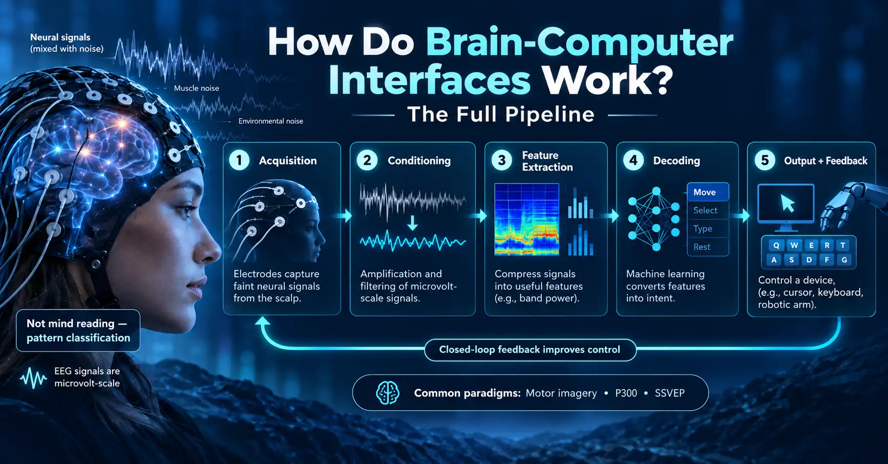
Your cortex produces electrical activity measured in millionths of a volt. Scalp EEG typically sits between minus 100 and plus 100 microvolts, with spatial resolution no finer than about 3 centimetres and a usable band of roughly 0 to 40 Hz, according to a comprehensive review in Frontiers in Neurorobotics. A fluorescent tube throws more electrical energy at the sensor than your intention does. So does a clenched jaw.
The machine, then, spends most of its effort not on understanding you. It spends it on finding you.
What a Brain-Computer Interface Actually Claims to Do
Strip out the marketing and a BCI makes a narrow claim. Give it a window of electrical activity and it will tell you which of a small set of pre-trained patterns that window most resembles.
That’s classification. It isn’t translation.
The difference matters more than anything else on this page. A translator maps open-ended input to open-ended output. A classifier picks from a menu somebody built in advance. When a user moves a cursor left, the system has not understood the concept “left”. It scored the incoming features against a pattern it learned earlier, while that same user imagined a left-hand movement, and left won the scoring.
Three signal paradigms carry most working systems:
- Motor imagery. You imagine moving a limb. Rhythms over sensorimotor cortex shift, and the decoder watches for that shift.
- P300. Your brain produces a positive voltage deflection roughly 300 milliseconds after a rare, relevant stimulus. Flash letters in a grid and that deflection fingerprints the one you were waiting for.
- SSVEP. Stare at a light flickering at 12 Hz and your visual cortex starts oscillating near 12 Hz. Flicker four buttons at four rates, then read the dominant frequency to know which button you chose.
Look at what those share. Each asks you to produce a signal the machine already knows how to recognise. The burden of being legible falls on you, not on the algorithm.
How Do Brain-Computer Interfaces Work? Five Stages, One Enemy
The chain runs like this:
- Acquisition. Electrodes convert ionic activity in tissue into a measurable voltage.
- Conditioning. Amplifiers lift that voltage; filters strip out everything that isn’t brain.
- Feature extraction. Software compresses the cleaned time series into a handful of numbers.
- Decoding. A trained model maps those numbers onto an intended action.
- Output and feedback. Something moves, and you watch it move.
Stages two through five all exist because stage one is bad at its job. If electrodes delivered clean, sharply localised neural activity, you could feed raw voltages to a simple threshold detector and go home. They don’t, so you can’t.
Stage 1: Getting a Signal Out of the Skull
An electrode does something less glamorous than it sounds. Neurons communicate with ion flows; electrodes conduct with electrons. The metal-tissue boundary is where one becomes the other, and that boundary is the noisiest, least stable part of the entire system.
Where you place the electrode sets the ceiling for everything downstream. Scalp EEG has to read through skin, muscle, and bone. Bone is a poor conductor, so it attenuates the signal and smears it sideways. That’s the physical origin of the 3-centimetre resolution limit: you aren’t measuring a neuron, or even a column of neurons. You’re measuring the blurred sum of a few square centimetres of cortex.
Move the sensor inward and the blur drops away.
- Subdural ECoG puts a grid of contacts directly on the cortical surface, beneath the skull. No bone in the path, so both spatial detail and usable bandwidth improve sharply.
- Intracortical arrays push microelectrodes into tissue, close enough to resolve the firing of individual neurons.
- Endovascular stent-electrodes thread a sensor through a blood vessel to sit against the vessel wall near motor cortex, which avoids opening the skull at all.
That last one matters because it breaks a binary the field argued about for years. A 2025 review of signal-acquisition methods sorts BCIs into three groups: non-implanted, interventional, and fully implanted. That’s a better map of where the hardware actually sits today than a straight invasive/non-invasive split.
Why Depth Buys Resolution, and What It Costs
Think of this as an engineering trade with a published price list. Every millimetre closer to the neurons buys fidelity and charges risk: surgery, infection, immune response, scar tissue that slowly degrades recording quality, and a device you can’t upgrade without another operation.
EEG charges you nothing surgically and hands you a smeared 3-centimetre picture. Intracortical arrays hand you single-neuron detail and charge you a craniotomy. Everything else lives between those poles. We’ve unpacked the sensor side of that argument in EEG vs fMRI vs ECoG, and the full risk calculus in invasive vs non-invasive BCIs.
One point gets lost in most comparisons. Resolution buys evidence, and evidence still has to be interpreted by something else. A better electrode hands the decoder a cleaner picture of the cortex. Working out what that picture means stays a separate problem, with its own separate failure modes.
Stage 2: Amplify First, Interpret Later
Analog-to-digital converters work in volts. Brains work in microvolts. Something has to bridge six orders of magnitude before a computer can do anything at all, and that something is the biopotential amplifier.
Its specifications tell you how hard the problem is. Input-referred noise has to stay under roughly 1 microvolt RMS, or the amplifier’s own thermal hiss drowns the cortex. Common-mode rejection ratio starts at 80 dB as a floor and reaches 100 to 110 dB in good commercial systems, according to Bitbrain’s engineering breakdown of EEG amplifier design.
That CMRR figure deserves a moment. Mains electricity radiates a 50 or 60 Hz field that hits both of your measurement points almost identically. A differential amplifier subtracts what the two inputs share and keeps only what differs. Rejecting 100 dB means suppressing that shared interference by a factor of 100,000. The building’s wiring is that much louder than your brain.
After amplification comes filtering. A band-pass filter discards frequencies outside the range of interest. A notch filter kills whatever mains hum survived the subtraction. Artifact rejection then removes the large, distinctive transients that eye movement and muscle tension produce.
Notice how unintelligent this whole stage is. Arithmetic and analog design, nothing more. And it’s where most cheap consumer headsets quietly fail.
Stage 3: Feature Extraction, or Deliberately Throwing Data Away
A clean signal is still the wrong shape for a classifier. A modest research rig — sixteen channels at 250 Hz — produces 4,000 numbers every second, almost all of them redundant. Feed that raw to a model and it will happily learn the room’s electrical quirks instead of your intent.
So the pipeline compresses. Established techniques include band power, amplitude measures, Hjorth parameters, autoregressive coefficients, and wavelet decompositions. Each one answers a specific question about the window: how much energy sits in the alpha band, how the signal’s complexity is changing, how well a short predictive model fits it.
That compression is where the real opinion lives.
Feature choice is a hypothesis. Picking band power over sensorimotor cortex encodes a claim about where imagined movement lives and what it looks like. If that claim is wrong for a particular user, no amount of downstream machine learning rescues the system. The decoder can only reason about what the features preserved, and the features already threw the rest away.
Stage 4: The Decoder, and Why It Only Knows You
Now machine learning finally enters. The decoder takes a feature vector and returns a class label, or a continuous value for something like cursor velocity. Classical statistical classifiers still do plenty of real work here. Deep networks take over where per-user data is plentiful enough to justify them. The architecture families we mapped out in ANN vs CNN vs RNN vs GNN show up here almost unchanged.
The interesting constraint sits upstream of the model choice. Nobody ships the decoder pre-trained.
Neural signatures vary enough between individuals that a population-average classifier underperforms one calibrated on a single person. So every BCI session opens with calibration: the user produces known intents on cue, the system records the matching neural activity, and the decoder fits itself to that labelled set. Signals also drift across sessions, as electrodes shift, impedance changes, and the user’s strategy evolves. Recalibration follows.
That’s the honest answer to why your BCI won’t just work out of the box. Brains differ from one another in ways the features can’t normalise away, so calibration survives every software release. A better version ships with the same opening chore attached.
“BCI Illiteracy” Is Really an Argument About Whose Fault It Is
Somewhere between 15 and 30% of people can’t produce a reliably classifiable signal with motor-imagery systems, even with off-the-shelf neuroimaging tools. The field used to call this BCI illiteracy, and increasingly calls it BCI inefficiency instead, as research on motor-imagery detection documents.
The rename carries an argument inside it. “Illiteracy” locates the deficit in the user, as though some brains simply can’t speak the language. “Inefficiency” locates it in the mismatch between that user’s neurophysiology and a decoder built around assumptions that don’t fit them.
Nobody has settled this. Both readings survive in the literature. How much of that 15 to 30% is fixed neurophysiology, and how much is bad algorithm-to-user matching, remains an open question. I lean toward the mismatch account, because the deficit model has a bad habit of hardening into a reason to stop investigating. But lean is the right word. The evidence doesn’t close the question.
Stage 5: Output, and the Loop That Trains Both Sides
Ask how do brain-computer interfaces work and most answers stop one stage short of here. Output looks trivial. A cursor moves, a letter appears, a robotic hand closes. Mechanically it’s the simplest step in the chain.
It’s also the one that makes the system work.
The moment a user sees the cursor respond, they’re inside a control loop. They adjust their strategy, and the decoder, if it keeps learning, adjusts alongside them. Research on closed-loop decoder adaptation shows that this simultaneous two-way adjustment produces better control than either a fixed decoder or a user learning alone against a static system.
That reframes the whole stack. The user belongs inside the algorithm, one adaptive component learning against another.
It also explains why demo videos mislead so reliably. A polished clip shows a trained user driving a decoder that has already co-adapted to them over hours or weeks. The same hardware, on a new person, on day one, behaves like a different product.
One Intended Movement, Traced End to End
Take a single action: a paralysed user intends to move a cursor to the right. Here’s what happens, in order.
- Intent. The user attempts the movement. Neurons in motor cortex fire in a population pattern associated with rightward reaching, regardless of whether any muscle can respond.
- Acquisition. An intracortical array picks up voltage fluctuations from tissue microns away, including spiking activity from individual neurons.
- Conditioning. Amplifiers raise microvolts to a usable range; filters remove mains interference and out-of-band content.
- Feature extraction. Software bins spike counts per electrode over a short window, typically tens of milliseconds, into a firing-rate vector.
- Decoding. A model trained during calibration maps that vector to a velocity in two dimensions: a direction and a speed, refreshed window after window.
- Output. The cursor moves. The user sees the error, adjusts their attempted movement, and the next window arrives a few tens of milliseconds later.
That loop repeats dozens of times a second. Recent intracortical cursor studies report calibration completing in under a minute, with control rates of several bits per second. That’s a genuine leap from where this work sat a decade ago.
It’s still a fraction of typing speed. And every one of those bits had to survive five stages of noise reduction to get there.
What This Pipeline Still Can’t Do
Any honest answer to how do brain-computer interfaces work has to include where they stop working. Accuracy varies sharply by paradigm, and the numbers are more modest than headlines suggest. The same Frontiers review reports P300 spellers reaching around 95%, SSVEP systems between 93 and 97%, and motor-imagery systems between 80 and 93%. It also warns that offline cross-validation accuracy tends to over-rate real-world online performance, which is a polite way of saying published figures flatter live systems.
Then there’s the vocabulary problem. A decoder only knows the classes it trained on. Intend something outside that set and the system doesn’t fail gracefully, it simply picks the nearest trained option. There’s no “I don’t know” button unless an engineer built one.
Recent intracortical speech work has demonstrated very high word accuracy across large vocabularies, which sounds like it breaks this limit. Look closer and it doesn’t. Those systems decode attempted speech, a motor act with a motor signature, from motor cortex. They aren’t tapping inner monologue. The distinction sounds pedantic until you consider what the difference means for anyone worried about what a BCI could be compelled to reveal.
Three things the current pipeline genuinely can’t do:
- Decode a thought it was never trained on.
- Work on a new user without calibration.
- Maintain constant performance across sessions without recalibration.
All three limits are structural. They live in the physics and the statistics of the stack, which is why they outlast product cycles.
The Honest Version Is More Interesting Than the Myth
“Brain implant reads minds” is a worse story than the truth. The truth runs like this. A few square centimetres of cortex leak a microvolt-scale whisper through bone. A chain of amplifiers, filters and classifiers then fights the building’s wiring for custody of that whisper. And a person on the other end slowly teaches a statistical model what their own intentions look like. Both of them get better at it together.
That’s a collaboration. Two learners, one slowly shared vocabulary. And it means the interesting ceiling on this technology may be neither electrode count nor model size. It may be how much time a human is willing to spend training a machine to recognise them.
Which raises the question worth sitting with. If the decoder only ever knows the version of you it was calibrated on, what happens on the day you change your mind about how to think?
Want the hardware half of that story next? Our EEG vs fMRI vs ECoG breakdown, linked above, is where I’d start.