

Type “a lighthouse in a storm, oil painting” into an image generator and watch what it doesn’t do. It doesn’t sketch. It doesn’t pick a palette or block out a composition. It starts with a rectangle of pure static and removes noise from it, again and again, until a lighthouse stands in the frame. So how do diffusion models work, if not by drawing? They learn one skill extremely well: undoing damage.
That skill sits underneath Stable Diffusion. It also raises a question this site keeps circling back to. When a machine produces something that no person made and no training image contains, who, or what, did the creating?
The mechanism is simpler than the output suggests. Music is messier than most explainers admit. And a 2025 study out of Stanford may have settled part of the creativity argument, though not the part most people care about.
What is a diffusion model, really?
A diffusion model is a generative model that learns to reverse a gradual noising process. It doesn’t produce an image in one shot. It gets there through many small corrections.
The modern version took shape in a June 2020 paper by Jonathan Ho, Ajay Jain and Pieter Abbeel, titled “Denoising Diffusion Probabilistic Models,” or DDPM. The authors described their approach as a “class of latent variable models inspired by considerations from nonequilibrium thermodynamics.” That’s physics language for something surprisingly intuitive.
The root idea is older. Jascha Sohl-Dickstein proposed it in 2015, borrowing from the way ink disperses in water. Drop ink into a glass and it spreads until the whole glass carries the same faint tint. That end state is boring. Boring turns out to be useful, because it’s easy to describe and easy to sample from.
Sohl-Dickstein put it vividly to Quanta Magazine: “The sequence of transformations very slowly turns your data distribution into just a big noise ball.” The “data distribution” here is simply the statistical shape of all the real images a model has seen. His insight was that if you learn the path into the noise precisely enough, you can walk it backward.
How do diffusion models work? Static in, structure out
Every diffusion model runs on two processes. One is dumb and fixed. The other is where all the intelligence lives.
Step one: ruin the data on purpose
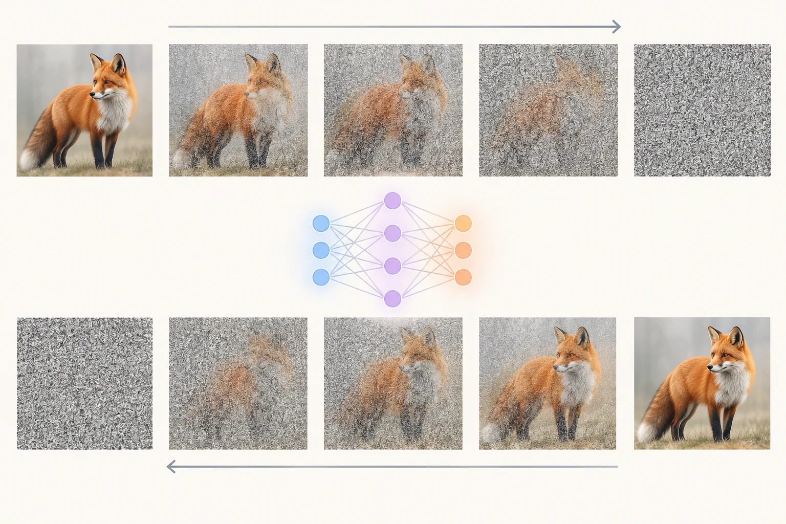
Training begins with destruction. Take a real image and add a little Gaussian noise, the fine random speckle you’d see on an old TV with no signal. Add a bit more. Keep going, step by step, until you can’t tell the picture apart from random noise.
Researchers call this the forward process. No learning happens here. It’s a fixed recipe, and that detail matters later, when we get to why diffusion won.
Step two: learn to undo it
The reverse process is where the neural network earns its keep. At each step, it looks at a noisy image and predicts what noise to remove. Not the whole answer. Just the next small cleanup.
Train that on enough images and something useful happens. Hand the network pure static it has never seen, ask it to clean up, and it keeps “finding” an image that fits the statistics of everything it learned. No picture hides in that static. The network builds one out of a long chain of guesses about what a slightly less noisy version should look like.
The most honest analogy is a sculptor who only knows one move: shaving off a sliver of stone. Repeat that move enough times, with good judgment about where to cut, and a statue appears. Nobody drew the statue first.
Even the early results were strong. The DDPM paper reported an FID of 3.17 on CIFAR-10, a standard benchmark of small images. FID measures how statistically close generated images are to real ones, and lower is better.
How text becomes a picture
Denoising static gets you an image. It doesn’t get you your image. Two more ideas turn a raw diffusion model into the text-to-image tool you’ve probably used.
Latent space: stop working on pixels
Early diffusion models worked directly on pixels, and that got expensive fast. Robin Rombach and his co-authors wrote that training powerful diffusion models in pixel space “often consumes hundreds of GPU days.” Their fix, which appeared in December 2021 and went on to CVPR 2022, was to compress first and denoise second.
An autoencoder squeezes each image into a much smaller “latent” representation that keeps what matters visually. The noising and denoising happen in that compact space. At the end, a decoder turns the finished latent back into pixels.
According to the latent diffusion paper, this move significantly reduced computational requirements while preserving visual fidelity. That’s the practical reason Stable Diffusion, which builds on this architecture, can run on consumer hardware with as little as about 2.4GB of video memory. It’s why you can watch how diffusion models work on your own graphics card instead of a rented server farm.
How your prompt steers the noise
The second idea is conditioning. Latent diffusion added cross-attention layers, which let a text encoder weigh in during denoising. Your prompt becomes a set of numbers. At every step, those numbers nudge the network’s guess about what to remove, pulling the result toward “lighthouse,” “storm” and “oil painting.”
That’s why prompting feels like steering rather than ordering. You aren’t specifying pixels. You’re tilting a long chain of tiny decisions in one direction, and the model fills in everything you didn’t say.

What it took to build Stable Diffusion
Stability AI released Stable Diffusion on August 22, 2022. The numbers behind version 1 give a sense of scale:
- An 860-million-parameter U-Net, the network that does the actual denoising
- A 123-million-parameter text encoder that turns your prompt into guidance
- Training data drawn from subsets of LAION-5B, a large image-text dataset
- 256 Nvidia A100 GPUs running for roughly 150,000 GPU-hours
- An estimated training cost of about $600,000
Six hundred thousand dollars is real money. By the standards of large AI models, though, it’s a modest bill, and the latent-space trick deserves much of the credit for keeping it there.
How the same idea reaches music (and where it doesn’t)
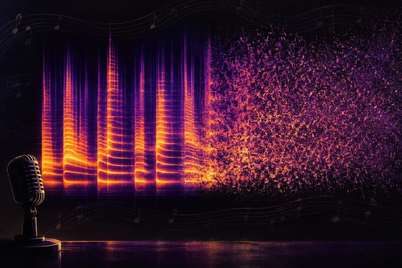
The noise-to-signal idea doesn’t care what the signal is. A diffusion model denoises whatever grid of numbers you give it. Sound can become such a grid: an audio spectrogram plots frequency against time, which makes a clip of music look a lot like an image.
So in principle, generating music can work exactly like generating a picture. Start from static and denoise toward something that matches the prompt.
Here’s the part most explainers skip. The best-documented text-to-music system of recent years, Google’s MusicLM, takes a different road. Its researchers cast text-to-music generation as a hierarchical sequence-to-sequence task. That’s closer in spirit to how large language models work than to how Stable Diffusion paints. The model builds a piece as a layered sequence rather than sculpting it out of noise.
The results are still striking:
- MusicLM produces continuous audio at 24 kHz that stays consistent over several minutes.
- Google trained it on roughly 280,000 hours of music.
- It can follow a hummed or whistled melody as well as a text description.
- Google also released MusicCaps, about 5.5k expert-annotated text-music pairs, to support future text-to-music research.
Why does the distinction matter? Because “AI music” isn’t one mechanism, and the honest answer to “how does it work” depends on which tool you mean. What unites these systems is a deeper move. They learn the statistics of an enormous body of human work, then generate new samples that fit those statistics. Diffusion is one road to that goal. Sequence modeling is another.
The MusicLM team also flagged a limitation worth sitting with. By their own check, roughly 1% of generated outputs closely resembled clips from the training data, and Google initially held back a public rollout. One percent sounds small until you ask whose recordings sit in that training set. That tension runs straight into the debate over AI music labeling and human authorship.
Why diffusion beat GANs
Before diffusion took over, the leading image generators were GANs, or generative adversarial networks. A GAN pits two networks against each other. One forges images; the other tries to catch the forgeries.
When a GAN works, it’s impressive. When it doesn’t, training wobbles or collapses, and the generator can settle into producing a narrow slice of outputs. That failure has a name: mode collapse.
Diffusion sidestepped the fight. It trains a single network against a fixed, well-behaved objective: predict the noise. No opponent, no arms race, and far fewer ways for training to go sideways. Remember that dumb, fixed forward process? This is where it pays off.
The decisive result came in May 2021. OpenAI researchers Prafulla Dhariwal and Alex Nichol published a paper with a blunt title: “Diffusion Models Beat GANs on Image Synthesis.” Using a technique called classifier guidance, their models reached:
- An FID of 3.94 on ImageNet at 256×256
- An FID of 3.85 on ImageNet at 512×512, with upsampling
- BigGAN-deep quality with as few as 25 forward passes per sample
They also covered the range of real images better than adversarial training did. Diffusion’s cost is that it works in steps, and each step means another full pass through the network. In 2021, twenty-five passes counted as quick.
If you want the family tree in one place, our comparison of GANs, VAEs and diffusion models puts all three side by side.
Is it creativity, or something else?
Here’s the puzzle that nagged at researchers. A diffusion model trained to reconstruct its data should, in theory, drift toward copies of what it saw. Instead, it keeps producing images that match no single training example. Where does that novelty come from?
In 2025, Stanford’s Mason Kamb and Surya Ganguli offered an answer that is almost deflating. They built a mathematical model, which they call the “equivariant local score” machine, with no training at all. It predicted what real diffusion models would output with 90% accuracy. Ganguli called that kind of result “unheard of in machine learning.”
Their model rests on two architectural constraints:
- Locality: the network works on small patches of an image rather than the whole scene at once.
- Translational equivariance: shift the input, and the output shifts the same way.
Both ideas will sound familiar if you’ve read our explainer on convolutional neural networks. Kamb summed up the finding to Quanta Magazine this way: “As soon as you impose locality, [creativity] was automatic; it fell out of the dynamics completely naturally.”
So, is it creative? Our read: the novelty is real, and the mystery isn’t. These systems stitch patch-level patterns into combinations nobody showed them. They do it because of their architecture, not because they understand or intend anything.
That’s a meaningful kind of generativity. It isn’t the kind of creativity that starts with wanting to say something. Whether human imagination secretly runs the same process at a larger scale is a question this research doesn’t answer, and shouldn’t have to.
What’s confirmed, and what’s still open
The site’s rule is to separate what we know from what we suspect. Here’s where things stand.
Confirmed by published research:
- Adding noise step by step and training a network to reverse it is the core of how diffusion models work (DDPM, 2020).
- Moving that process into a compressed latent space cut compute enough to put image generation on consumer hardware (latent diffusion, 2021–2022).
- Diffusion with classifier guidance beat the strongest GANs on ImageNet image quality (2021).
- A training-free model predicted real diffusion outputs with 90% accuracy by modeling locality and equivariance (2025).
Still open or debated:
- Whether diffusion or sequence modeling will prove the better route for music. MusicLM shows the second path works; the first remains possible in principle.
- How much resemblance to training data is acceptable. MusicLM’s roughly 1% near-copy rate was enough to slow its release.
- Whether “creativity” is even the right word for a process that has no goal beyond fitting the statistics.
What you’re actually looking at
Next time an image resolves out of static on your screen, remember what just happened. No one imagined it. A network made a long series of small, statistically confident guesses about what a slightly cleaner picture should look like, steered by your words.
That’s less magical than the marketing and more interesting than the dismissals. Knowing how diffusion models work doesn’t settle whether the output is art. It does sharpen the real question: when a machine’s guess lands close to something a person made first, whose work are we looking at?