
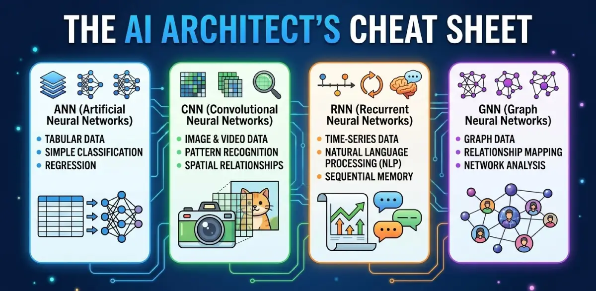
Choosing between ANN, CNN, RNN, and GNN gets much easier once you stop asking which acronym is ‘more advanced’ and start asking how your data is organized. This guide gives you a practical selection rule. If your signal lives in fixed feature vectors, start with a feedforward ANN. If it lives in local spatial patterns, use a CNN. If order across time is the main signal, an RNN or one of its gated variants makes sense. If the task depends on entities plus relationships, consider a GNN. By the end, you should be able to map a problem to the right neural network family, explain the tradeoff clearly, and avoid the common architecture mistakes that waste time.
Start with data topology, not model names
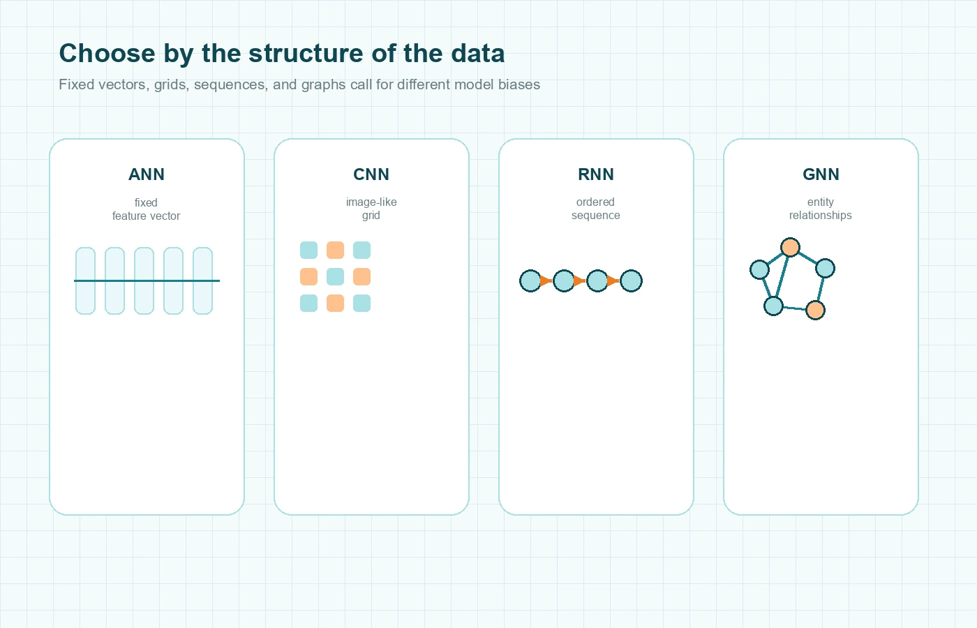
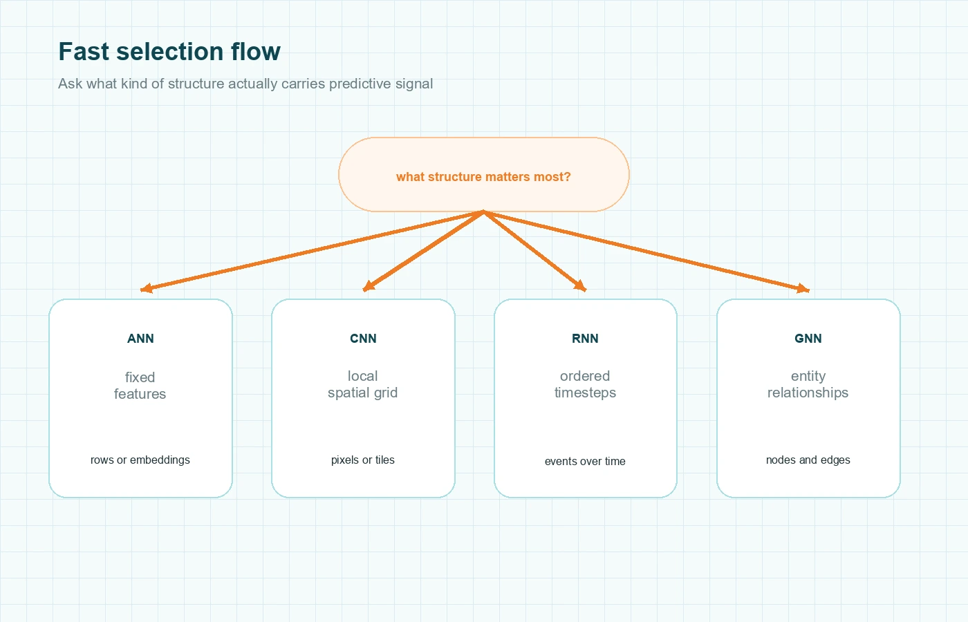
The fastest way to choose among these four architectures is to look at the shape of the information that carries the signal. A plain ANN works when each example is already a fixed-size feature vector. A CNN works when nearby values in a grid matter, such as pixels in an image. An RNN works when order matters across a sequence of steps. A GNN works when entities and their relationships matter together.
That framing is not just a teaching shortcut. It follows the way the architectures are built. CS231n’s neural network notes explain feedforward models as layered functions over vectors. Its convolution notes focus on local receptive fields and shared weights for image-like data. Its recurrent notes describe models that carry state across ordered inputs. Distill’s GNN introduction explains why graphs are different: their size and connectivity can vary from example to example.
Think about one product with four different data sources. A risk platform may have a borrower profile as tabular data, document images from uploaded statements, a sequence of past transactions, and a network linking accounts, devices, merchants, and IP addresses. That is one business problem, but it contains four different structure types. The best architecture depends on which structure drives the prediction you care about.
This is also where architecture debates often go wrong. Teams compare models as if they were general-purpose rivals, when the real question is whether the model’s built-in assumptions match the data.
When a plain ANN is the right tool
In this comparison, ANN is best treated as the feedforward baseline, sometimes called a multilayer perceptron. It is the right place to start when every example can be represented as one stable vector of features and the relationships between examples are not the main story.
Imagine a churn model that uses account age, subscription tier, average weekly usage, ticket count, and region. Each customer can be expressed as one row of numbers or encoded categories. A feedforward network can learn non-linear combinations across those features without needing spatial filters, recurrent state, or graph message passing.
This is the sweet spot for a plain ANN: structured tabular data, fixed-size embeddings, engineered features from upstream systems, and baseline classifiers or regressors where structure-specific inductive bias is not required. The advantage is simplicity. You do not have to preserve pixel neighborhoods, sequence order, or graph edges. That usually makes the data pipeline cleaner and the baseline easier to debug.
There is also a strategic reason to start here. If your task performs well with a strong feedforward baseline, you may not need a more specialized model. For many business problems, the expensive mistake is not using an ANN. It is adding architectural complexity before proving the structure matters.
Where does ANN become the wrong abstraction? Images are the clearest example. If you flatten a 256 x 256 image into one long vector, the model loses the idea that neighboring pixels are near each other. Graph problems fail in a similar way. If you collapse a fraud network into isolated rows, you remove the relational context that may carry the strongest signal.
If you want the deeper foundation first, MindoxAI’s guide to artificial neural networks is the right supporting explainer.
When to use CNN
A convolutional neural network is a better fit when local spatial patterns repeat across a grid. Images are the classic case, but the deeper reason is worth stating plainly: CNNs assume that nearby values matter together and that the same kind of pattern can appear in different positions.
CS231n’s convolution notes explain this with local connectivity and shared weights. The AlexNet paper is the famous proof point that this design became extremely effective for large-scale vision tasks.
Suppose you are building a defect detector for manufactured parts. A scratch in the top-left corner and a scratch in the bottom-right corner are still scratches. You want a model that can learn an edge, texture, or small shape once and reuse that knowledge anywhere in the image. That is exactly what convolution gives you.
CNNs are usually the right fit when the input is an image or image-like grid, local patterns matter more than absolute position alone, translation invariance is useful, and feature learning should happen from raw spatial data rather than hand-built features. This is why CNNs also show up beyond natural photos. Spectrograms, medical scans, satellite tiles, and some time-series representations can benefit from convolution when local neighborhoods matter.
The common misuse is treating CNNs as a generic upgrade over ANNs. They are not automatically better. If your input is already a clean feature table, adding convolution can create structure that is not really there. Convolution helps because it matches the data topology, not because it is more fashionable.
MindoxAI’s standalone explainer on convolutional neural networks is a strong internal follow-up for readers who want to go deeper on filters and feature maps.
When to use RNN
An RNN is built for ordered data. The key word is ordered, because not every dataset with timestamps or rows is truly sequence-dependent. You use a recurrent model when the meaning of the current step depends on what came before it.
CS231n’s RNN notes frame recurrent networks around hidden state, which is simply a running summary carried from one step to the next. That makes them useful when you care about evolving context rather than one static snapshot.
Take a machine-monitoring example. A single temperature reading may look normal. A rising pattern across the last twenty readings may not. A recurrent model can process the stream in order and let earlier signals influence the present prediction. The same logic applies to language. In the phrase ‘the server was overloaded, so traffic was…’ the next word depends on the earlier sequence, not on isolated tokens.
RNNs are a good fit when sequence order is part of the signal, the model should update its state step by step, streaming or online inference matters, and nearby or medium-range context influences the prediction. That is why they still make sense for event streams, sensor data, and other sequence-first tasks.
This is also the section where many articles get vague. They say RNNs have memory, then immediately admit vanilla RNNs struggle with long dependencies. Both statements are true. Recurrent models can carry context forward, but training becomes harder as the chain gets longer. Pascanu, Mikolov, and Bengio explain the exploding- and vanishing-gradient problem directly, and that is one reason LSTM and GRU variants became so important.
So the practical rule is simple. If your problem is sequence-first, an RNN family model makes sense. If your task is really about spatial neighborhoods or graph relationships, forcing it into a recurrent pipeline is usually a design smell.
Readers who want the longer version can branch into MindoxAI’s guide to recurrent neural networks.
When to use GNN
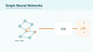
Graph neural networks are the right choice when the thing you want to predict depends on both entity features and the links between entities. If edges are not just metadata but part of the signal, that is where GNNs begin to earn their complexity.
Distill’s introduction to graph neural networks is the clearest practical explanation of why graphs need a different architecture. A graph is not a fixed grid. One node might connect to two neighbors, another to two thousand. That irregularity makes standard feedforward or convolutional assumptions a poor fit.
The central idea is message passing. In plain language, a node updates its representation by combining its own features with information from connected neighbors. The Neural Message Passing paper made that framing especially influential. Later variants changed how the aggregation worked. GCN popularized a practical convolution-style update on graphs. GraphSAGE focused on inductive learning over large, evolving graphs. GAT introduced attention so some neighbors could matter more than others.
Picture a fraud system instead of a molecule paper. Accounts, devices, merchants, phone numbers, and IP addresses can all become nodes. Connections between them may reveal suspicious rings that no isolated row of features captures. Two transactions might look harmless alone but become suspicious when they sit inside a dense, repeated pattern of shared devices and money flows.
GNNs are a good fit when the input is naturally a graph, neighborhood context is predictive, node, edge, or whole-graph predictions matter, and new information arrives as relationships rather than just new columns. They are not free wins. Graph construction is hard, noisy edges can hurt, and deeper graph stacks can over-smooth node representations. A GNN is powerful when the graph is real. It is overkill when the graph is artificial, weak, or built mostly because the team wants to use a modern architecture.
For the architecture-specific deep dive, MindoxAI already has a strong primer on graph neural networks.
ANN vs CNN vs RNN vs GNN cheat sheet
Here is the shortest useful version of the comparison.
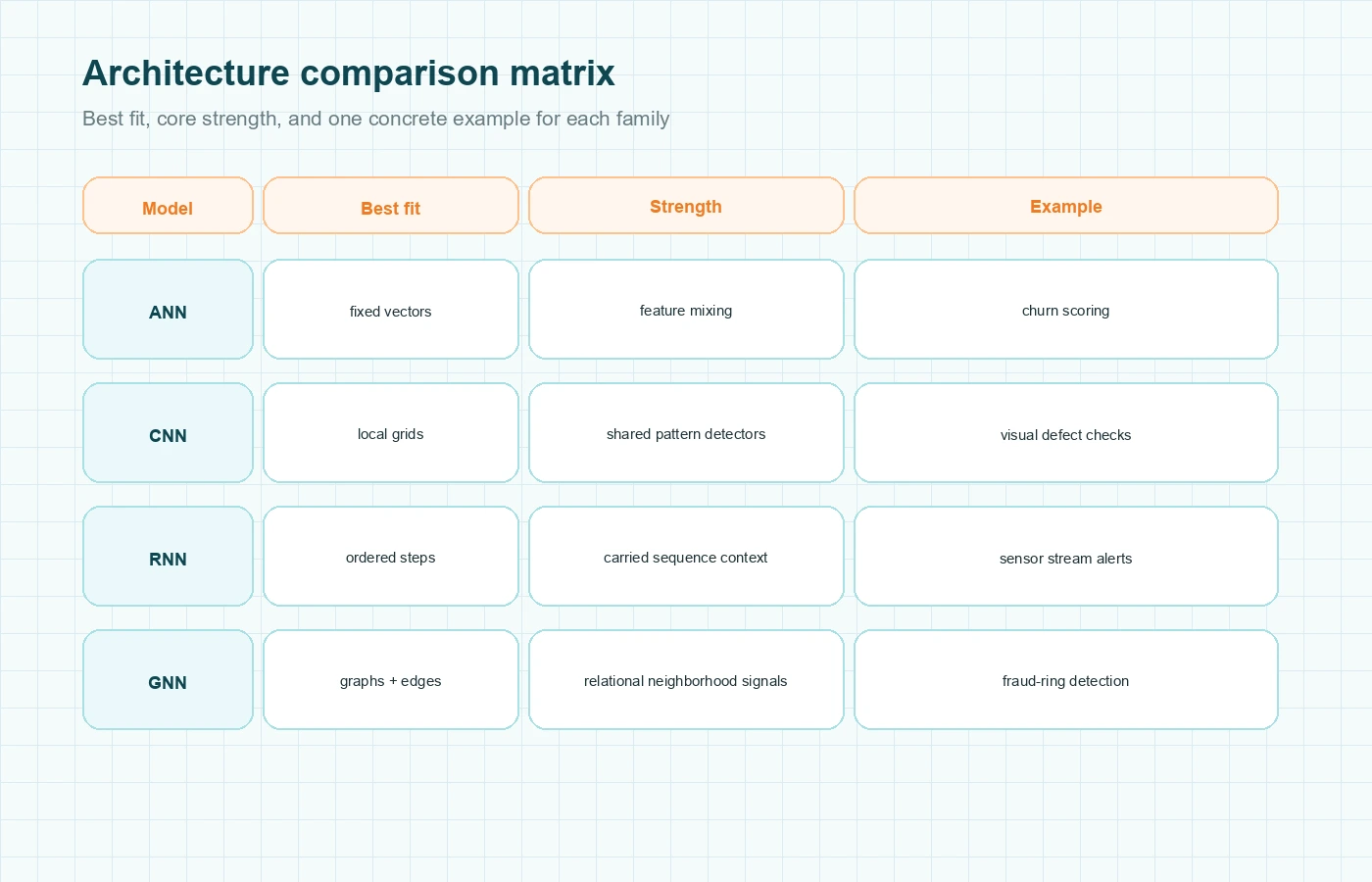
| Architecture | Best-fit data shape | What it exploits | Concrete example | Common wrong move |
|---|---|---|---|---|
| ANN | Fixed-size feature vector | Non-linear combinations of features | Churn prediction from customer attributes | Flattening images or graphs and pretending structure does not matter |
| CNN | Grid or local neighborhood structure | Repeating local spatial patterns | Defect detection on part images | Using convolution on data with no meaningful spatial locality |
| RNN | Ordered sequence | Context carried across timesteps | Sensor-stream anomaly detection | Treating independent samples as if they were a sequence |
| GNN | Graph of entities and edges | Attributes plus relational neighborhood | Fraud-ring detection or molecule property prediction | Building a graph without proving the edges add signal |
You can also reduce the choice to four short questions. Is each example already a stable feature vector? Start with ANN. Does local spatial layout carry the signal? Use CNN. Does reordering the input change the meaning? Use RNN. Do explicit relationships between entities change the answer? Use GNN.
That rule is simple, but it is not simplistic. It lines up with the assumptions built into the architectures themselves.
Common architecture selection mistakes
The first mistake is choosing by hype instead of by structure. Teams sometimes jump to GNN because the problem sounds complex, or to CNN because the model feels more advanced than a feedforward network. That is backward. The model should follow the structure that carries predictive signal.
The second mistake is confusing storage format with learning structure. A time series stored in a CSV file is still sequential data. A graph stored in edge tables is still graph data. The file format does not decide the model family.
Another failure mode is underestimating hybrids. A recommendation system might use a CNN to embed product images, an ANN on tabular merchant features, and a GNN over the user-item interaction graph. A monitoring product might use an RNN over event streams and a GNN over machine dependencies. The right question is not always which one wins. Sometimes it is which subsystem needs which bias.
The last mistake is skipping the baseline. If an ANN on well-prepared features is already strong, that tells you something important about the problem. Specialized architectures should earn their complexity by capturing structure the baseline cannot.
Final Thoughts
If you remember one rule from this article, make it this: choose the model that matches the dominant structure of the signal. Fixed vectors point toward ANN. Grids point toward CNN. Ordered steps point toward RNN. Real relationships between entities point toward GNN.
That framing is more useful than memorizing acronyms. It gives you a way to explain architecture choice, spot mismatches early, and build a better baseline before the project gets expensive.